Getting started with EUBUCCO

curl --progress-bar -C - -o CH04.parquet "https://s3.eubucco.com/eubucco/v0.2/buildings/parquet/nuts_id=CH04/CH04.parquet"

# Alternatively, use the AWS CLI to download the file:
aws s3 cp s3://eubucco/v0.2/buildings/parquet/nuts_id=CH04/CH04.parquet . \
    --endpoint-url https://s3.eubucco.com \
    --no-sign-request

import geopandas as gpd

gdf = gpd.read_parquet("CH04.parquet")

import geopandas as gpd

region = "CH04"
s3_path = f"s3://eubucco/v0.2/buildings/parquet/nuts_id={region}/{region}.parquet"
storage_opts = {
    "anon": True,
    "client_kwargs": {"endpoint_url": "https://s3.eubucco.com"}
}

gdf = gpd.read_parquet(s3_path, storage_options=storage_opts)

import duckdb

con = duckdb.connect()
con.execute("INSTALL httpfs; LOAD httpfs;")
con.execute("INSTALL spatial; LOAD spatial;")

# Specify the S3 endpoint 
con.execute("SET s3_endpoint='s3.eubucco.com';") 
con.execute("SET s3_url_style='path';")
con.execute("SET s3_region='eu';")
con.execute("SET s3_access_key_id='';")
con.execute("SET s3_secret_access_key='';")

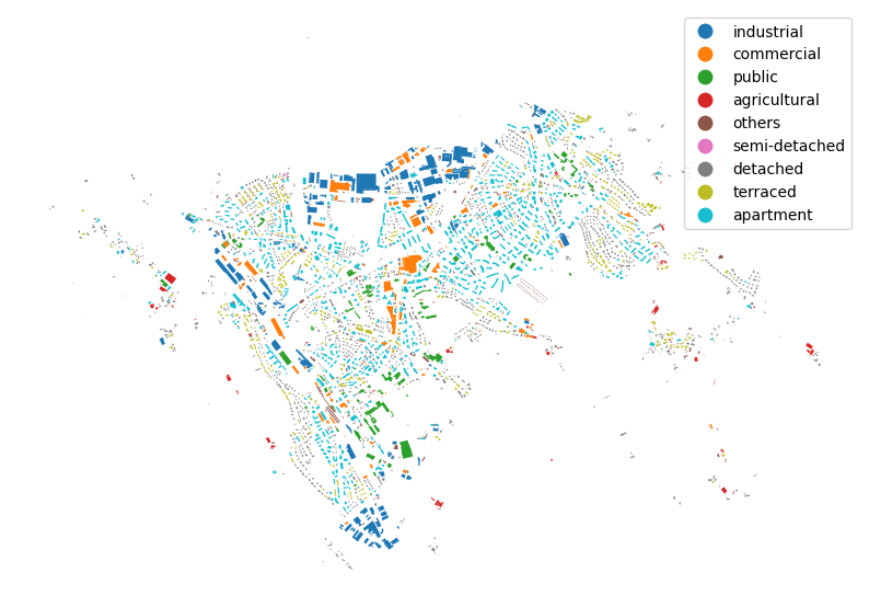
import geopandas as gpd

# Fetch data with WKB-encoded geometries
region = "CH04"
s3_path = f"s3://eubucco/v0.2/buildings/parquet/nuts_id={region}/{region}.parquet"
query = f"""
    SELECT * EXCLUDE geometry, ST_AsWKT(geometry) AS geometry
    FROM '{s3_path}' 
"""
df = con.execute(query).df()

# Convert to GeoDataFrame
gdf = gpd.GeoDataFrame(
    df,
    geometry=gpd.GeoSeries.from_wkt(df["geometry"]),
    crs="EPSG:3035",
)

gdf["country"] = gdf["region_id"].str[:2]  # EU VAT 2-digit country code
gdf["NUTS1"] = gdf["region_id"].str[:3]  # EU NUTS1 code
gdf["block_id"] = gdf["id"].str.split("-").str[0]  # Identify touching buildings

gdf["type_is_authoritative"] = gdf["type_source"].str.contains("gov")  # Identify buildings with authoritative type information
gdf["type_is_merged"] = (gdf["geometry_source"] != gdf["type_source"]) & (gdf["type_source"] != "estimated")  # Identify buildings with merged type information
gdf["type_is_estimated"] = gdf["type_source"] == "estimated"  # Identify buildings with estimated type information
gdf["type_is_inferred"] = gdf["geometry_source"] != gdf["type_source"]  # Identify buildings with type being merged or estimated

city = gdf[gdf["city_id"] == "CHCH0121"]
city.plot(column="subtype", legend=True, figsize=(10, 8)).set_axis_off()

city = gdf[gdf["city_id"] == "CHCH0247"]
city["height"] = city["height"].astype(float)
city[["id", "height", "height_source", "geometry"]].explore(
    column="height",
    cmap="YlOrRd",
    tiles="CartoDB positron",
    legend=True,
)

gov = gdf[~gdf["geometry_source"].isin(["osm", "msft"])]
gov[["id", "geometry_source"]].sample(3)

ground_truth_height = gdf[gdf["height_source"] != "estimated"]
ground_truth_height[["id", "height", "height_source"]].sample(3)

# Categorical: Correct type in >80% of cases
reliable_type = gdf[gdf["type_confidence"].fillna(1.0) > 0.8]

# Numerical: Precise height (uncertainty interval < 2m)
precise_height = gdf[(gdf["height_confidence_upper"] - gdf["height_confidence_lower"]).fillna(0.0) < 2.0]
precise_height[["id", "height", "height_source", "height_confidence_lower", "height_confidence_upper"]].sample(3)

# Extract buildings in France taller than 50m
s3_path = "s3://eubucco/v0.2/buildings/parquet/*/*.parquet"
query = f"""
    SELECT *
    FROM read_parquet('{s3_path}', hive_partitioning = true)
    WHERE nuts_id LIKE 'FR%' AND height > 50
    LIMIT 10
"""
df = con.execute(query).df()
df[["id", "region_id", "height"]]

# Extract buildings within bounding box (bbox needs to be in EPSG:3035)
s3_path = "s3://eubucco/v0.2/buildings/parquet/*/*.parquet"
query = f"""
    SELECT *
    FROM read_parquet('{s3_path}', hive_partitioning = true)
    WHERE bbox.xmin >= 5300000 AND bbox.xmax <= 5400000
    AND bbox.ymin >= 1880000 AND bbox.ymax <= 1920000
    LIMIT 10
"""
df = con.execute(query).df()
df[["id", "region_id", "subtype", "height", "geometry_source"]]

# Count governmental buildings across Europe
s3_path = "s3://eubucco/v0.2/buildings/parquet/*/*.parquet"
query = f"""
    SELECT
        count(*) AS gov_count,
        LEFT(region_id, 2) AS country
    FROM read_parquet('{s3_path}', hive_partitioning = true)
    WHERE geometry_source NOT IN ('msft', 'osm')
    GROUP BY country
    ORDER BY gov_count DESC
"""
count = con.execute(query).df()
count

stats = gpd.read_parquet("region-stats.parquet")

country_stats = stats.drop(columns=["geometry", "region_id", "region_name"]).groupby("country").sum()
country_stats[["n_gt_type", "n_gt_subtype", "n_gt_height", "n_gt_floors", "n_gt_construction_year"]].div(country_stats["n"], axis=0).rename(columns=lambda x: x.replace("n_gt_", "share_gt_")).round(2)

stats["height_coverage"] = stats["n_gt_height"] / stats["n"]

tooltip = [
    "n",
    "n_gov",
    "n_osm",
    "n_msft",
    "n_gt_type",
    "n_gt_subtype",
    "n_gt_height",
    "n_gt_floors",
    "n_floors_0_3",
    "n_floors_4_6",
    "n_floors_7_inf",
    "n_type_residential",
    "n_type_non_residential",
]
stats["n"] = stats["n"].div(1000).round()
stats.explore(
    "n",
    legend=True,
    tiles="CartoDB positron",
    cmap="Blues",
    legend_kwds={"caption": "Number of Buildings (in thousands)"},
    tooltip=tooltip,
)

# Simple aggregated visualization with H3 hexagons
import h3pandas

gdf_floor = gdf[["geometry", "height"]].copy()
gdf_floor["height"] = gdf_floor["height"].astype(float)
gdf_floor["floor_area"] = ((gdf_floor.area * gdf_floor["height"]) / 1000 / 1000).round(2)
gdf_floor["geometry"] = gdf_floor.centroid.to_crs("EPSG:4326")
h3_grid = gdf_floor.h3.geo_to_h3_aggregate(resolution=8, operation="sum")

# precision
h3_grid.explore(
    column="floor_area",
    cmap="YlGn",
    tiles="CartoDB positron",
    tooltip=["floor_area"],
    legend=True,
)

con.execute("INSTALL h3 FROM community; LOAD h3;")
s3_path = "s3://eubucco/v0.2/buildings/parquet/*/*.parquet"
h3_resolution = 5

query = f"""
WITH buildings AS (
    SELECT
        height,
        ST_Transform(
            ST_Point(
                (bbox.ymin + bbox.ymax) / 2,
                (bbox.xmin + bbox.xmax) / 2
            ),
            'EPSG:3035',
            'EPSG:4326'
        ) AS centroid
    FROM read_parquet('{s3_path}', hive_partitioning = true)
    WHERE height IS NOT NULL
    LIMIT 1000000 -- comment out to run query at scale
),

h3_stats AS (
    SELECT
        h3_latlng_to_cell_string(
            ST_X(centroid),
            ST_Y(centroid),
            {h3_resolution}
        ) AS h3,
        AVG(height) AS avg_height,
        COUNT(*) AS n_buildings
    FROM buildings
    GROUP BY h3
)

SELECT
    h3,
    avg_height,
    n_buildings,
    h3_cell_to_boundary_wkt(h3) AS geometry
FROM h3_stats
"""

df = con.execute(query).df()

h3_grid = gpd.GeoDataFrame(
    df,
    geometry=gpd.GeoSeries.from_wkt(df["geometry"]),
    crs="EPSG:4326",
)

h3_grid[h3_grid["n_buildings"] > 100].explore(
    column="avg_height",
    vmax=20,
    cmap="YlOrRd",
    tiles="CartoDB positron",
    legend=True,
    tooltip=["avg_height", "n_buildings"],
)